Histograms Are Used to Display Quantitative and Continuous Data
One to one maths interventions built for KS4 success
Weekly online one to one GCSE maths revision lessons now available
Learn more
This topic is relevant for:

Histogram
Here we will learn about histograms, including how to draw a histogram and how to interpret them.
There is also a histogram worksheet based on Edexcel, AQA and OCR exam questions, along with further guidance on where to go next if you're still stuck.
What is a histogram?
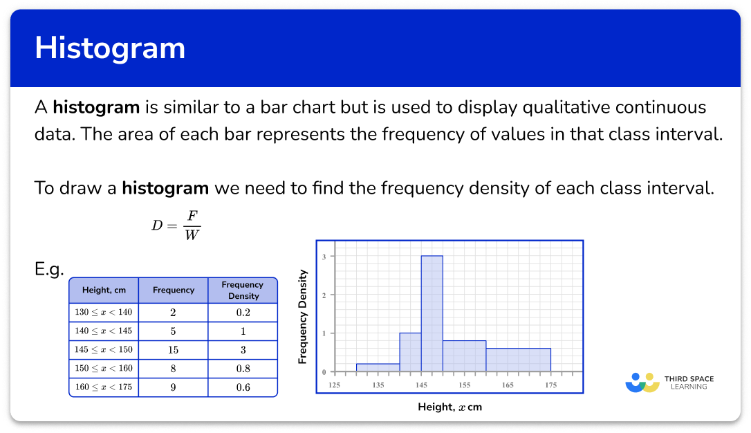
A histogram is similar to a bar chart but is used to display quantitative continuous data (numeric data), whereas a bar chart (or bar graph) is used to display qualitative or quantitative discrete data.
In a bar chart, the heights of the bars represent the frequencies, whereas in a histogram the area of the bars represent the frequencies.
To draw a histogram we need to find the frequency density of each class interval.
The frequency density (D) of a class interval is equal to the frequency (F) divided by the class width (W).
Expressing this as a formula, we have
D=\frac{F}{W} .
These values are then used for the heights of the bars on the vertical axis ( y -axis).
The horizontal axis ( x -axis) is labelled as the data variable with a continuous scale (not grouped).
For example,
Below is a grouped frequency table and the associated histogram.

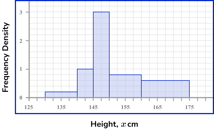
Notice that the class intervals do not have to be the same size for a histogram. This means that the class width (W) may be different for each bar. Do not assume it is the same value for the data set.
A histogram can be used to show the shape of a frequency distribution of a data set.
Analysing the distribution of data is an important skill and is looked at in more depth in A Level Mathematics.
Step-by-step guide: Frequency density
Step-by-step guide: Frequency density formula
What is a histogram?
How to draw a histogram
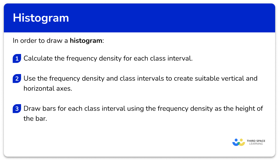
In order to draw a histogram:
- Calculate the frequency density for each class interval.
- Use the frequency density and class intervals to create suitable vertical and horizontal axes.
- Draw bars for each class interval using the frequency density as the height of the bar.
Explain how to draw a histogram
Histogram worksheet
Get your free histogram worksheet of 20+ questions and answers. Includes reasoning and applied questions.
DOWNLOAD FREE
Histogram worksheet
Get your free histogram worksheet of 20+ questions and answers. Includes reasoning and applied questions.
DOWNLOAD FREE
Histogram examples
Example 1: drawing a histogram from grouped data
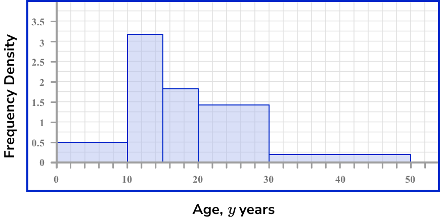
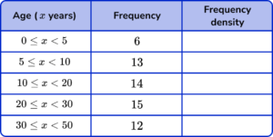
The table shows information about the ages of people at a cinema.
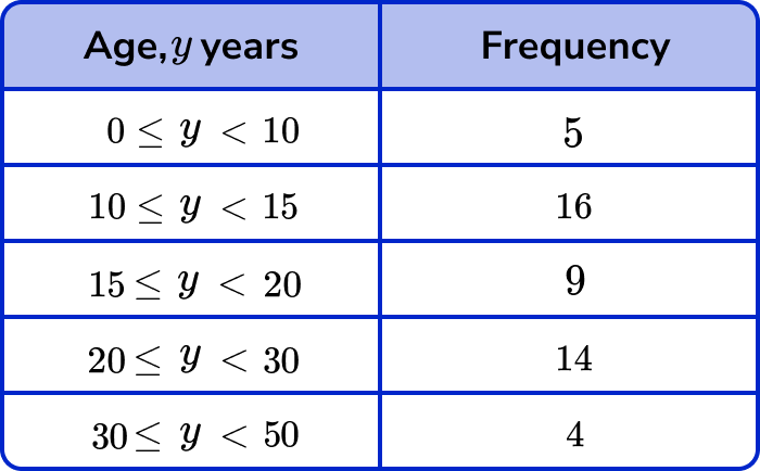
Use the information in the table to draw a histogram.
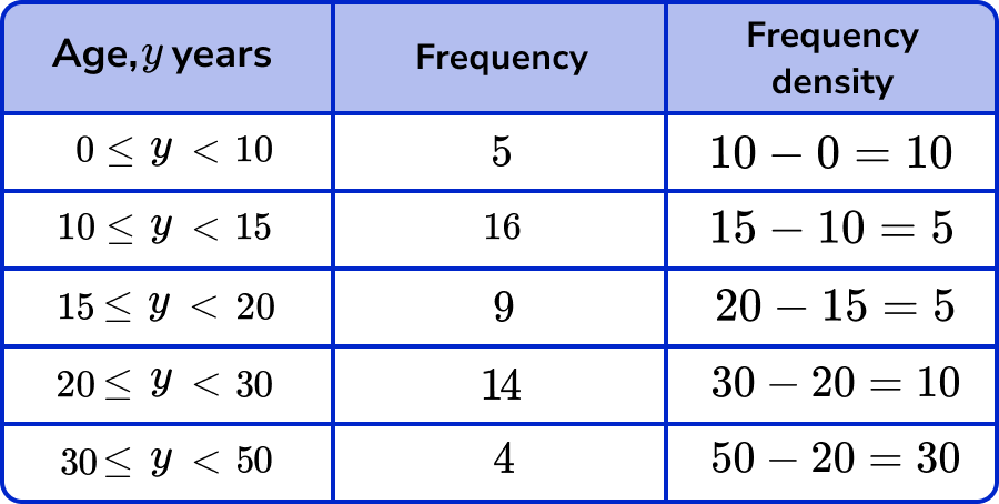
- Calculate the frequency density for each class interval.
First we need to calculate the class width for each row. This is the highest value in the range, subtracting the lowest value in the range.
Here we have
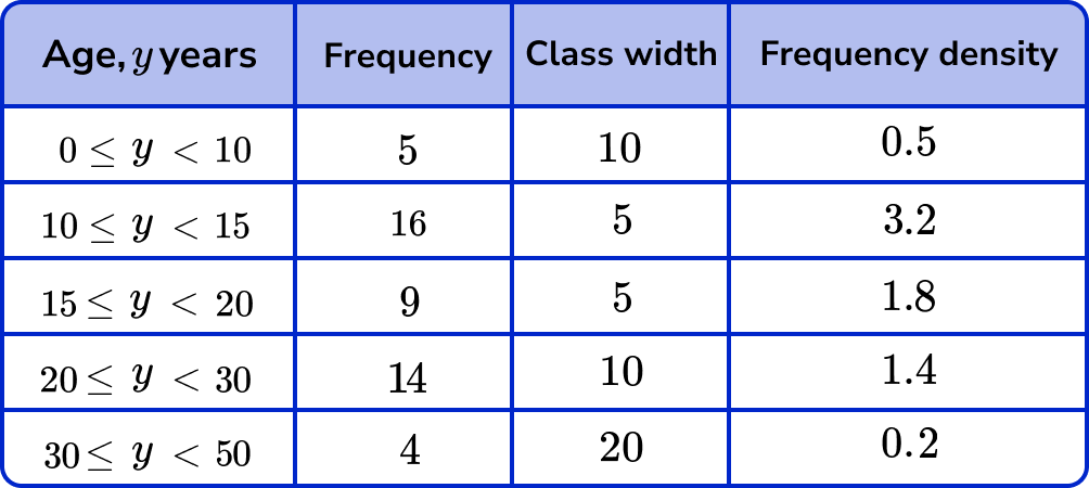
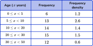
Now we know the class width, we can calculate the frequency density using the formula D=\frac{F}{W} .
For the first row, F=5 and W=10 so D=\frac{5}{10}=0.5.
For the second row, F=16 and W=5 so D=\frac{16}{5}=3.2.
Continuing this for the rest of the table, we have
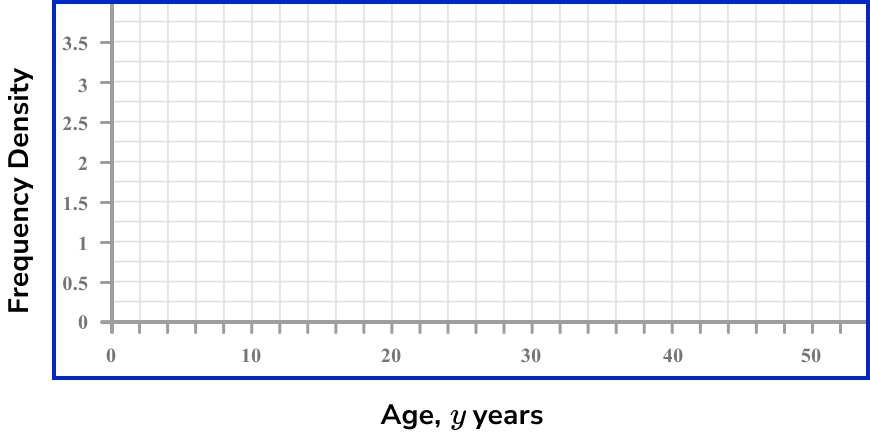
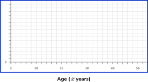
2 Use the frequency density and class intervals to create suitable vertical and horizontal axes.
The maximum frequency density is 3.2 and the horizontal scale needs to go from 0 to 50.
3 Draw bars for each class interval using the frequency density as the height of the bar.
Make sure you use a pencil and a ruler to draw each bar with precision.
Example 2: drawing a histogram from grouped data
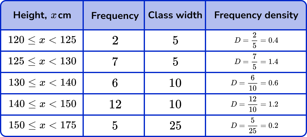
The table shows information about the heights of pupils in a mathematics class.

Use the information to construct a histogram.
Calculate the frequency density for each class interval.
Using the frequency density formula D=\frac{F}{W}, we substitute the information from each row to calculate the frequency density. Remember to calculate the class width for each class.
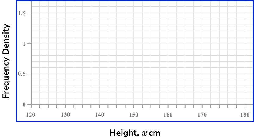
Use the frequency density and class intervals to create suitable vertical and horizontal axes.
The maximum frequency density is 1.4 and the horizontal scale needs to go from 120 to 175.
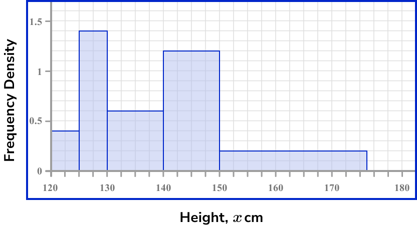
Draw bars for each class interval using the frequency density as the height of the bar.
Drawing each bar one after the other with no gaps, we have
Example 3: drawing a histogram from grouped data
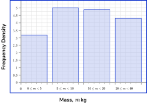
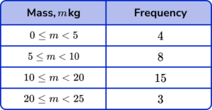
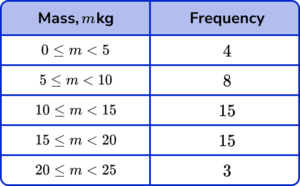
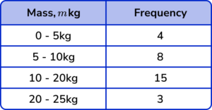
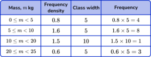
The table shows information about the mass of fish in a lake.
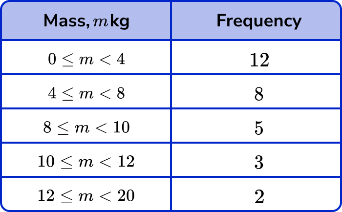
Use the information to construct a histogram.
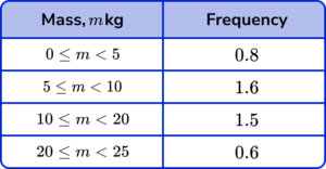
Calculate the frequency density for each class interval.
Using the frequency density formula, we have
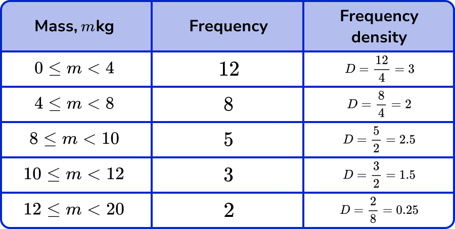
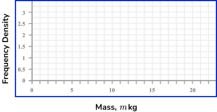
Use the frequency density and class intervals to create suitable vertical and horizontal axes.
The maximum frequency density is 3 and the horizontal scale needs to go from 0 to 20.
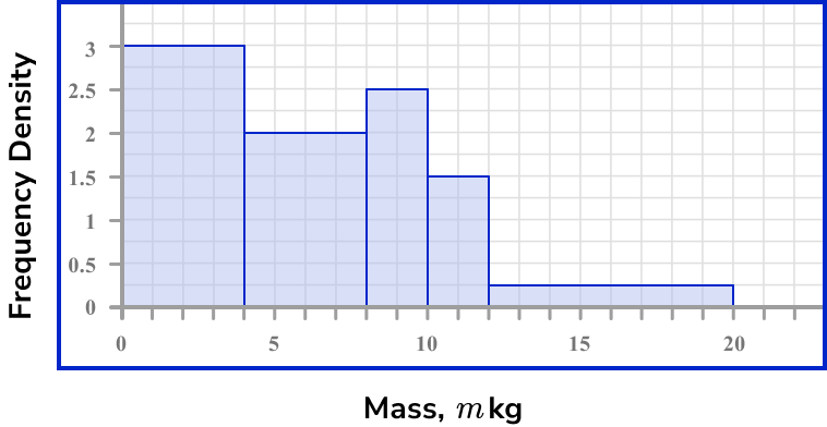
Draw bars for each class interval using the frequency density as the height of the bar.
How to calculate frequency from a histogram
In order to calculate frequency from a histogram:
- Locate the frequency density for the class interval(s).
- Determine the class width for the class interval(s).
- Use the frequency density formula to determine the frequency.
Explain how to calculate frequency from a histogram
Calculating frequency examples
Example 4: calculating the frequency of a class interval from a histogram
The histogram below show information about the height h of plants in a garden.
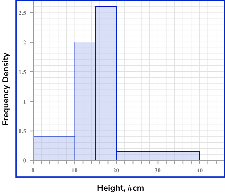
Calculate the frequency of values in the interval 0 \leq h < 10.
Locate the frequency density for the class interval(s).
We need to use the histogram to obtain this value for the class. The vertical axis is the frequency density and so we need to read this value for the first bar.
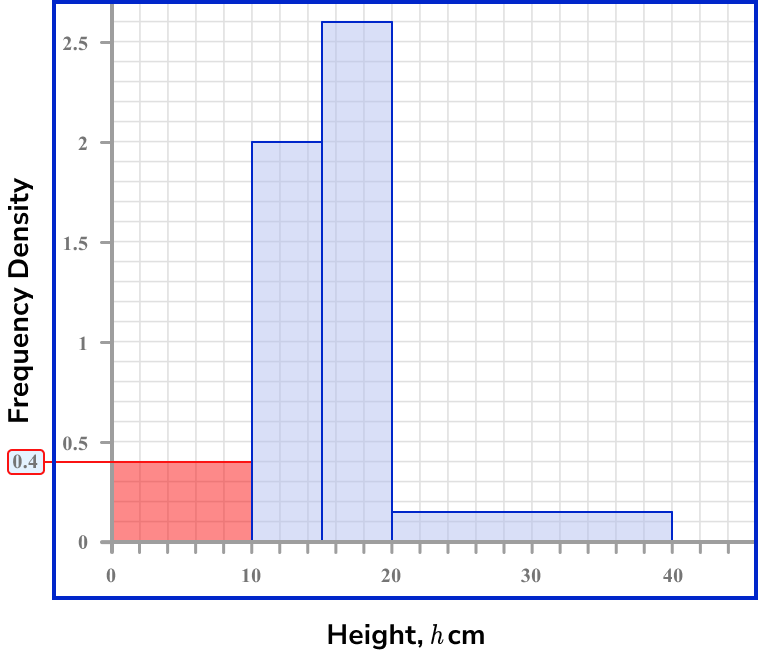
The frequency density for the first class interval is D=0.4.
Determine the class width for the class interval(s).
The interval 0 \leq h < 10 has a class width W=10-0=10.
Use the frequency density formula to determine the frequency.
The frequency density formula is D=\frac{F}{W}.
As D=0.4 and W=10, we can substitute these values into the formula and solve for F.
\begin{aligned} 0.4&=\frac{F}{10}\\\\ 0.4\times{10}&=F\\\\ F&=4 \end{aligned}
The frequency of plants in the interval 0 \leq h < 10 is 4.
Example 5: calculating the frequency of a class interval from a histogram
The histogram below shows information about the time t seconds taken for students to complete a 400m race.
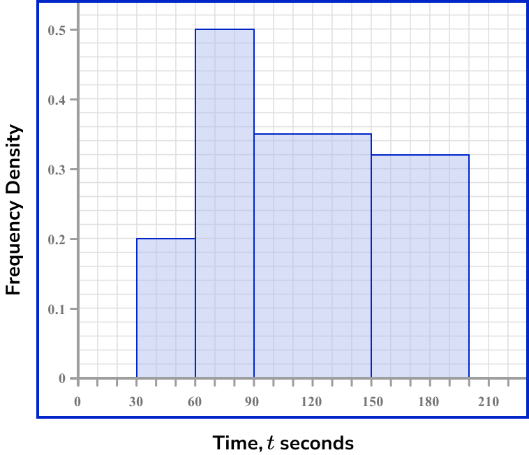
How many students ran 400m in under 90 seconds?
Locate the frequency density for the class interval(s).
We need to use the histogram to obtain this value for each class under 90 seconds. This would be the first two class intervals.
The vertical axis is the frequency density and so we need to read this value for the first and second bars.
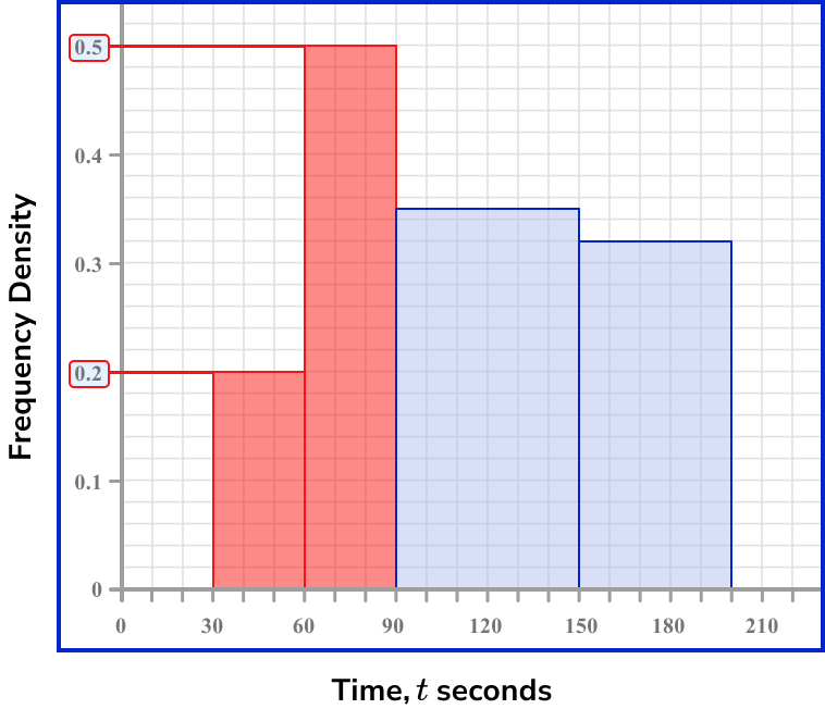
The frequency density for the class interval 30 \leq t < 60 is D=0.2.
The frequency density for the class interval 60 \leq t < 90 is D=0.5.
Determine the class width for the class interval(s).
The interval 30 \leq t < 60 has a class width W=60-30=30.
The interval 60 \leq t < 90 has a class width W=90-60=30.
Use the frequency density formula to determine the frequency.
To calculate the frequency in both of these class intervals, we must work out the frequency in each class separately, then add them together at the end.
The frequency density formula is D=\frac{F}{W}.
As D=0.2 and W=30, for the interval 30 \leq t < 60, we can substitute these values into the formula and solve for F.
\begin{aligned} 0.2&=\frac{F}{30}\\\\ 0.2\times{30}&=F\\\\ F&=6 \end{aligned}
As D=0.5 and W=30, for the interval 60 \leq t < 90, we can substitute these values into the formula and solve for F.
\begin{aligned} 0.5&=\frac{F}{30}\\\\ 0.5\times{30}&=F\\\\ F&=15 \end{aligned}
The frequency of students who ran 400m in under 90 seconds is 15 + 6 = 21 students.
Example 6: calculating the frequency of a random interval from a histogram
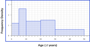
The histogram below shows information about the age of children who participated in a research study about mental health.
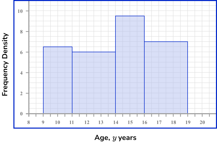
Estimate the number of students between 12 and 14 years old who participated in the research study.
Locate the frequency density for the class interval(s).
The frequency density for students aged between 12 and 14 years old is the same height. This means that the frequency density is the same for all students between this age range.
The vertical axis is the frequency density and so we need to read this value for the interval of 12 to 14 years.
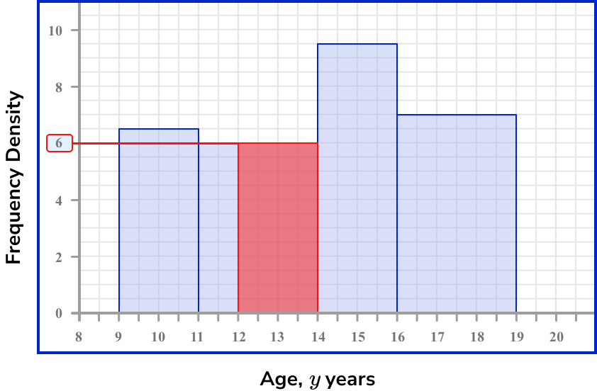
The frequency density for the interval is D=0.6.
Determine the class width for the class interval(s).
As we have an age range of 12 to 14 years, the class width is W=14-12=2 .
Use the frequency density formula to determine the frequency.
To calculate the frequency we use the frequency density formula.
D=\frac{F}{W}
As D=6 and W=2 for the age range of 12 to 14 years, we substitute these values into the formula and solve for F.
\begin{aligned} 6&=\frac{F}{2}\\\\ 6\times{2}&=F\\\\ F&=12 \end{aligned}
An estimate for the frequency of students between 12 and 14 years old who participated in the study is 12.
Common misconceptions
- Frequency vs frequency density
A very common error that occurs in histogram questions is that the frequency is used instead of the frequency density. Frequency density must be found because the groups provided in the frequency table are usually not equal width.
- The height of the bar is the frequency, instead of the area
Similar to the previous misconception, the height of the bar is considered to be the frequency whereas it is the area of the bar that represents the frequency for a histogram.
- The horizontal axis is labelled as discrete groups, rather than a continuous scale
The horizontal axis of a bar chart is divided into discrete categorical variables with gaps between the bars. This knowledge is incorrectly transferred to histograms. A histogram plots values on a continuous scale and so there are no gaps between classes.
Practice histogram questions


Frequency density is used for the height of the bars of a histogram.
\text{Frequency density }=\frac{\text{class width}}{\text{frequency}}
\text{Frequency density }=\frac{\text{frequency}}{\text{midpoint}}
\text{Frequency density }=\frac{\text{frequency}}{\text{class width}}
\text{Frequency density }=\frac{\text{cumulative frequency}}{\text{class width}}
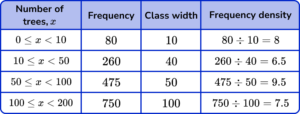
The frequency density is the frequency per unit for the data in each class interval.
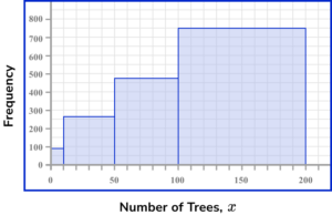

Calculating the frequency density for each row using the formula D=\frac{F}{W}, we have
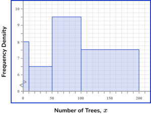
The horizontal axis of a histogram should be labelled with the variable (here, the number of trees x ) using a continuous scale. Each bar should be the width of the interval. The scale should range from 0 to 200.
The vertical axis is labelled frequency density. Each bar should be drawn up to the frequency density value for the class. There must not be a break in the vertical axis. The scale should range from 0 to 10 minimum.
This produces the histogram.


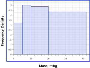
Calculating the frequency density for each row using the formula D=\frac{F}{W}, we have
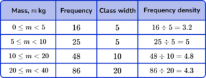
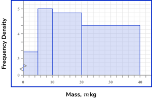
The horizontal axis of a histogram should be labelled with the variable (here, the Mass, m \ kg ) using a continuous scale. Each bar should be the width of the interval. The scale should range from 0 to 40.
The vertical axis is labelled frequency density. Each bar should be drawn up to the frequency density value for the class. There must not be a break in the vertical axis. The scale should range from 0 to 5 minimum.
This produces the histogram.
The frequency table must contain the correct frequencies for each class. The class intervals are determined by the location of the start and end of the bar on the horizontal scale, so the first class would have the interval 0 \leq m <5 as the edges of the bar are at 0kg and 5kg.
The range must allow all values between the limits with no duplicate values for the mass.
The frequencies are calculated by finding the area of each bar (multiplying the height by the width). Specifically, this is found by multiplying the class width by the frequency density for each bar.
The frequency is the area of the bar for the given interval. The width of the bar is from 10:00am to 10:20am and so this could be considered as 20 minutes, or W=20. The height of the bar (the frequency density) is D=1.4 for the whole interval.
The frequency is therefore
\begin{aligned} F&=D\times{W}\\\\ F&=1.4\times{20}\\\\ F&=28 \end{aligned}
Histogram GCSE questions
1. (a) The frequency table shows the ages of guests at a hotel.
Complete the 'Frequency density' column of the table.
(b) Use the table to draw a histogram for the data. Use the axes provided below.
(6 marks)
Show answer
(a)
Attempt to divide frequency by class width seen.
(1)
Minimum of 3 of the frequency density values correct.
(1)
All frequency density values correct.
(1)
(b)
Frequency density used for vertical scale.
(1)
3 bars correct.
(1)
All bars correct.
(1)
2. The histogram shows information about the mass of 20 newborn calves on a farm.
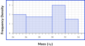
Use the histogram to estimate the number of calves with a mass of more than 31 \ kg.
(3 marks)
Show answer
Area of the fourth bar ( 32 to 24kg ) =2 \times 1.5=3 .
(1)
Area of bar within the range of 31 to 22 =1 \times 3=3 .
(1)
Frequency =6
(1)
3. The widths of plant stems in a garden were collected. An incomplete histogram and associated table are shown below.
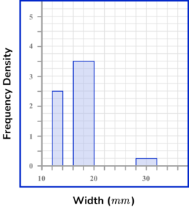
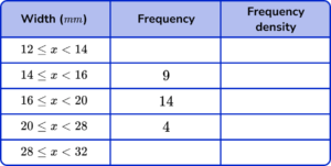
Use the information provided to complete the histogram and table.
(5 marks)
Show answer
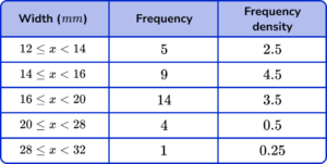
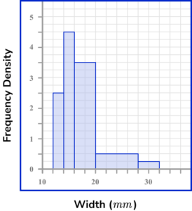
Frequency density of the class 16 \leq x <20 is 3.5 .
(1)
Frequency density of the class 12 \leq x <14 is 2.5
and
Frequency of the class 12 \leq x <14 is 2.5 \times 2 = 5 .
(1)
Frequency density of the class 28 \leq x <32 is 0.25
and
Frequency of the class 28 \leq x <32 is 0.25 \times 4 = 1 .
(1)
Frequency density of the class 14 \leq x <16 is 9 \div 2 = 4.5
and
Drawn correctly on the histogram.
(1)
Frequency density of the class 20 \leq x <28 is 4 \div 8 = 0.5
and
Drawn correctly on the histogram.
(1)
Learning checklist
You have now learned how to:
- Construct and interpret diagrams for grouped discrete data and continuous data, i.e. histograms with equal and unequal class intervals and cumulative frequency graphs, and know their appropriate use
Beyond GCSE
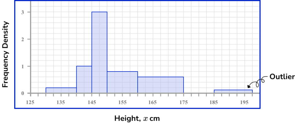
Histograms are used extensively beyond GCSE, below are a few examples.
It is often quite easy to spot outliers on a histogram. This is because there may be an individual data point shown in a small bar that is located separate to the main data set which does not fit the general trend in the data.
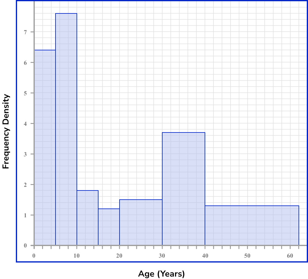
A histogram is bimodal when there are two clusters of data within one data set. This would look like two peaks within the histogram and would occur if the majority of data lies in two separate groups.
For example, if you collected data on the ages of people who watched a young children's film at the cinema, you are likely to have a lot of young children, accompanied by adults and so fictitiously, there would be fewer teenagers attending this viewing at the cinema, leaving a dip in the middle of the data.
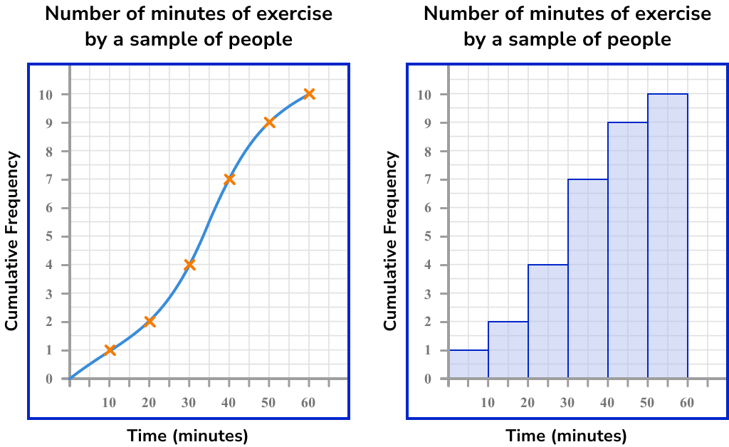
A cumulative histogram plots the cumulative number of observations in each bin, up to a specified bin. This would look similar to a cumulative frequency curve but represented using bars, instead of a line.
When we look at very large samples of data, the majority of the data usually lies in the middle of the range of values, with fewer values as we get further away from the median.
If we constructed a histogram with equal class sizes (sometimes known as bin widths) that represented the heights of the population of a country, you would get the approximate visualisation,
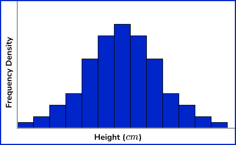
Here, the bar with the highest frequency is the central bar, with the frequency of each bar decreasing as it gets further away from the centre. If we highlighted the mean, mode and median on this diagram, they would occur in the same place,
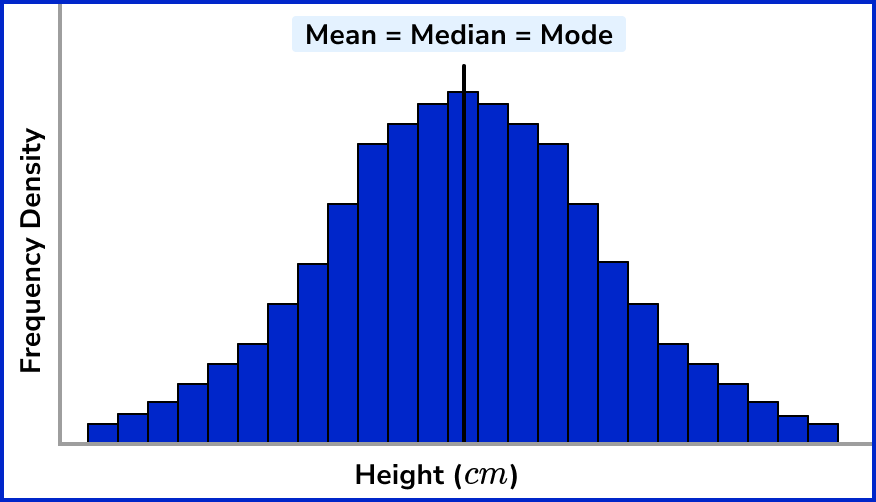
If we decrease the width of each class size (the bin sizes) by increasing the number of classes (the number of bins*), the histogram would tend towards a curved bell shape that is symmetric about the mean,
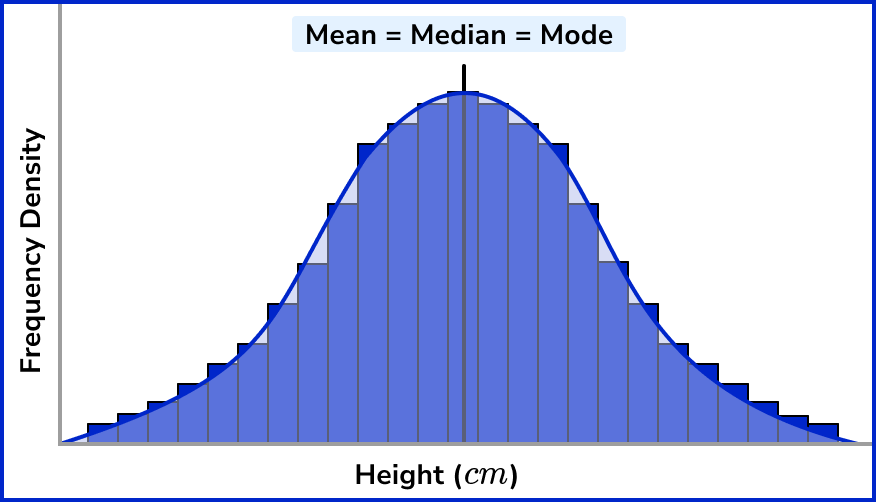
*The optimal number of histogram bins can be determined using Sturges formula.
This bell curve is the shape of the normal distribution, with mean μ. The standard deviation σ is the spread of the data from the mean. The higher the value for the standard deviation, the more spread out the data is relative to the mean.
Here, one standard deviation for the blue curve is larger than one standard deviation for the red curve,
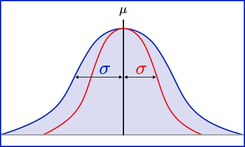
The standard deviation is the square root of the variance (the average degree to which each data value varies from the mean).
The empirical rule states that 68\% of the data values lie within 1 standard deviation of the mean, 95\% of data values lie within 2 standard deviations of the mean and 99.7\% of data following a normal distribution lies within 3 standard deviations of the mean.
If we took a sample of the population, Scott's normal reference rule is the standard deviation of the sample.
The normal distribution is used a lot in probability theory, where the probability density function defines the shape of the distribution, here, the normal distribution with a bell shaped curve.
If the bell shaped curve was asymmetric about the mean, the degree of skewness can be measured from a positive skew, to a negative skew.
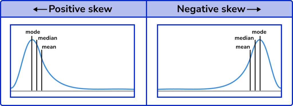
Outliers can impact the skewness of a set of data as they still exist within the sample or population but the majority of the data would be distributed away from this value (someone may be very good at holding their breath for a significant length of time, whereas the majority of the population data would be in a much smaller range – an example of positive skew).
- For positive skew: mode < median < mean
- For no skew: mode = median = mean
- For negative skew: mean < median < mode
Still stuck?
Prepare your KS4 students for maths GCSEs success with Third Space Learning. Weekly online one to one GCSE maths revision lessons delivered by expert maths tutors.
Find out more about our GCSE maths revision programme.
We use essential and non-essential cookies to improve the experience on our website. Please read our Cookies Policy for information on how we use cookies and how to manage or change your cookie settings.Accept
salisburyguick1946.blogspot.com
Source: https://thirdspacelearning.com/gcse-maths/statistics/histogram/
0 Response to "Histograms Are Used to Display Quantitative and Continuous Data"
Post a Comment